Coupling Navier-Stokes and Gross-Pitaevskii equations for the numerical simulation of two-fluid quantum flows | LMRS Numerical Methods and Applications Group

Download preprint-pdf

Authors

M. Brachet, G. Sadaka, Z. Zhang, V. Kalt and I. Danaila

Abstract

Numerical methods for solving the Navier-Stokes equations for classical (or normal) viscous fluids are well established. This is also the case for the Gross-Pitaevskii equation, governing quantum inviscid flows (or superfluids) in the zero temperature limit. In quantum flows, like liquid helium II at intermediate temperatures between zero and 2.17 K, a normal fluid and a superfluid coexist with independent velocity fields. The most advanced existing models for such systems use the Navier-Stokes equations for the normal fluid and a simplified description of the superfluid, based on the dynamics of quantized vortex filaments, with ad hoc reconnection rules. There was a single attempt (C. Coste, 1998) to couple Navier-Stokes and Gross-Pitaevskii equations in a global model intended to describe the compressible two-fluid liquid helium II. We present in this contribution a new numerical model to couple a Navier-Stokes incompressible fluid with a Gross-Pitaevskii superfluid. Coupling terms in the global system of equations involve new definitions of the following concepts: the regularized superfluid vorticity and velocity fields, the friction force exerted by quantized vortices to the normal fluid, the covariant gradient operator in the Gross-Pitaevskii model based on a slip velocity respecting the dynamics of vortex lines in the normal fluid. A numerical algorithm based on pseudo-spectral Fourier methods is presented for solving the coupled system of equations. Finally, we numerically test and validate the new numerical system against well-known benchmarks for the evolution in a normal fluid of different types or arrangements of quantized vortices (vortex crystal, vortex dipole and vortex rings). The new coupling model has the advantage to keep the full Gross- Pitaevskii model for the superfluid, and thus describe quantized vortex dynamics without any phenomenological approximation. This opens new possibilities to revisit and enrich existing numerical results for complex quantum fluids, such as quantum turbulent flows.

Supplemental material: 2D superfluid vortex dipole

Test Case	Parameters
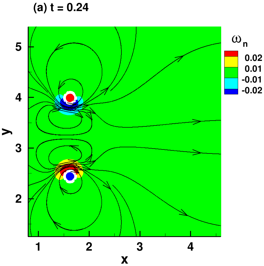
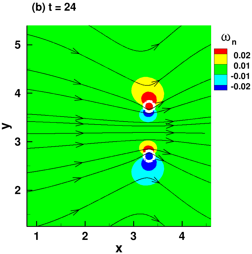
2D evolution of a superfluid vortex dipole. Two-way GP-NS coupling. Illustration of the triple-vortex structure of the flow. The entrained normal fluid is represented by its vorticity contours (colors) and streamlines (arrow black lines). Superfluid vortices (white circles) are identified by an iso-contour of low atomic density (0.5 $\|\psi\|^2_{max}$)	$B_{tab} = 0.4$, $B’_{tab} = 0.1$ $\eta_D=0$, $d/\xi = 53$ $N = 256$, $k_{\rm reg}^{-1}=\xi$
Snapshots of the flow for $t=0.24$	Snapshots of the flow for $t=24$

Supplemental material: 3D superfluid vortex ring

Test Case	Parameters
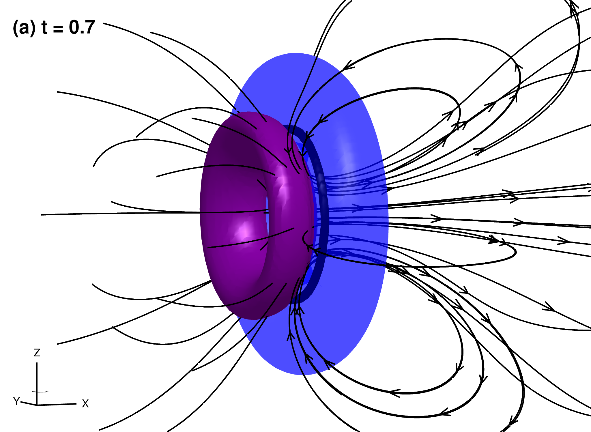
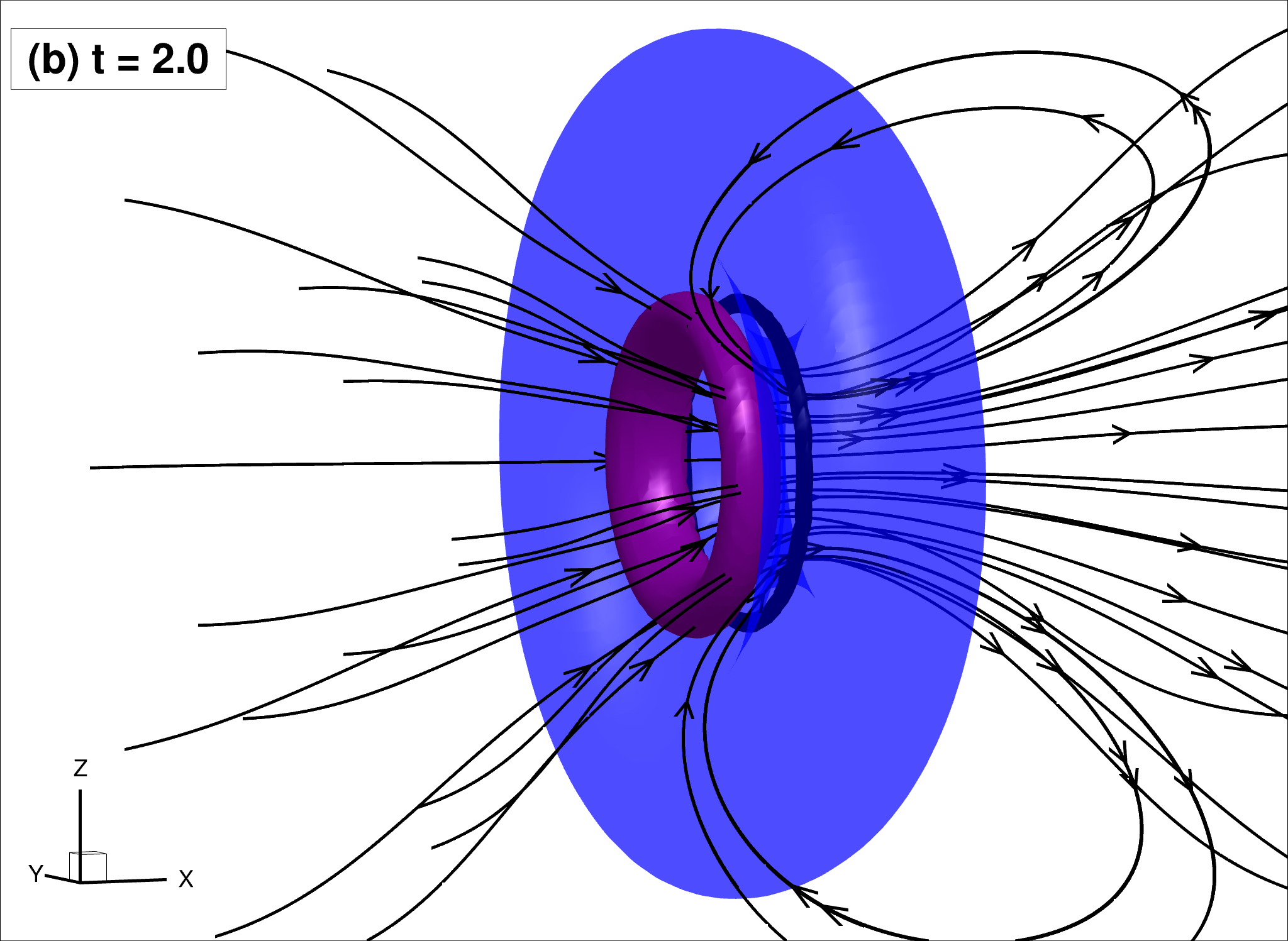
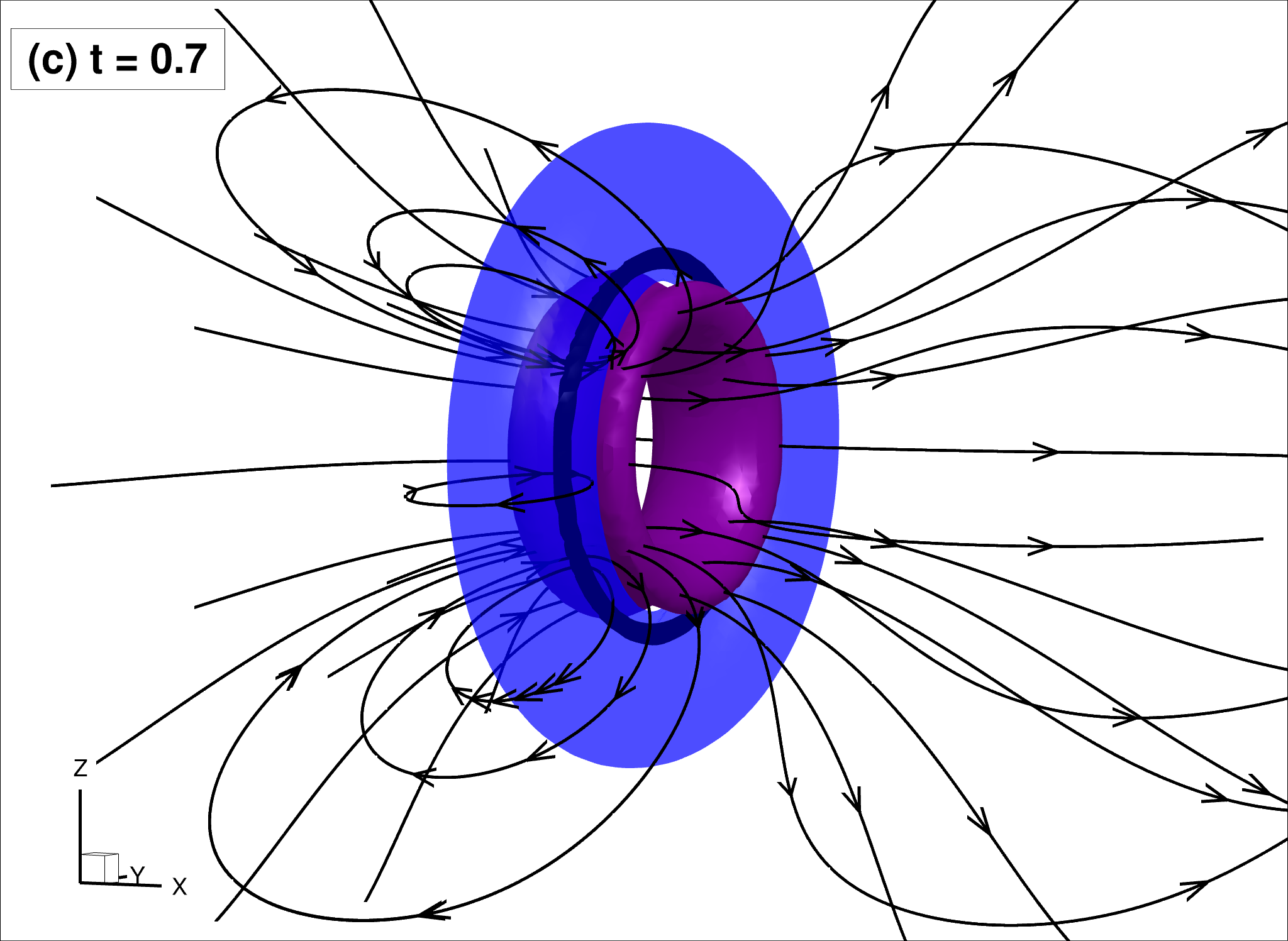
3D evolution of a superfluid vortex ring in a normal fluid initially at rest. Illustration of the triple-vortex structure. The superfluid vortex ring (in black) is identified by an iso-surface of low atomic density (0.5 $\|\psi\|^2_{max}$). The two counter-rotating normal vortex rings are identified by iso-surfaces of normal fluid azimuthal vorticity: $0.03$ for the blue outer ring and ($-0.03$) for the red inner ring. The streamlines in the normal fluid are also drawn	$\rho_n/\rho_s = 1$ $B_{tab}=B’_{tab} = 0.4$ $\eta_D=0.035B_{tab}$
Snapshots of the flow for $t=0.7$	Snapshots of the flow for $t=2$
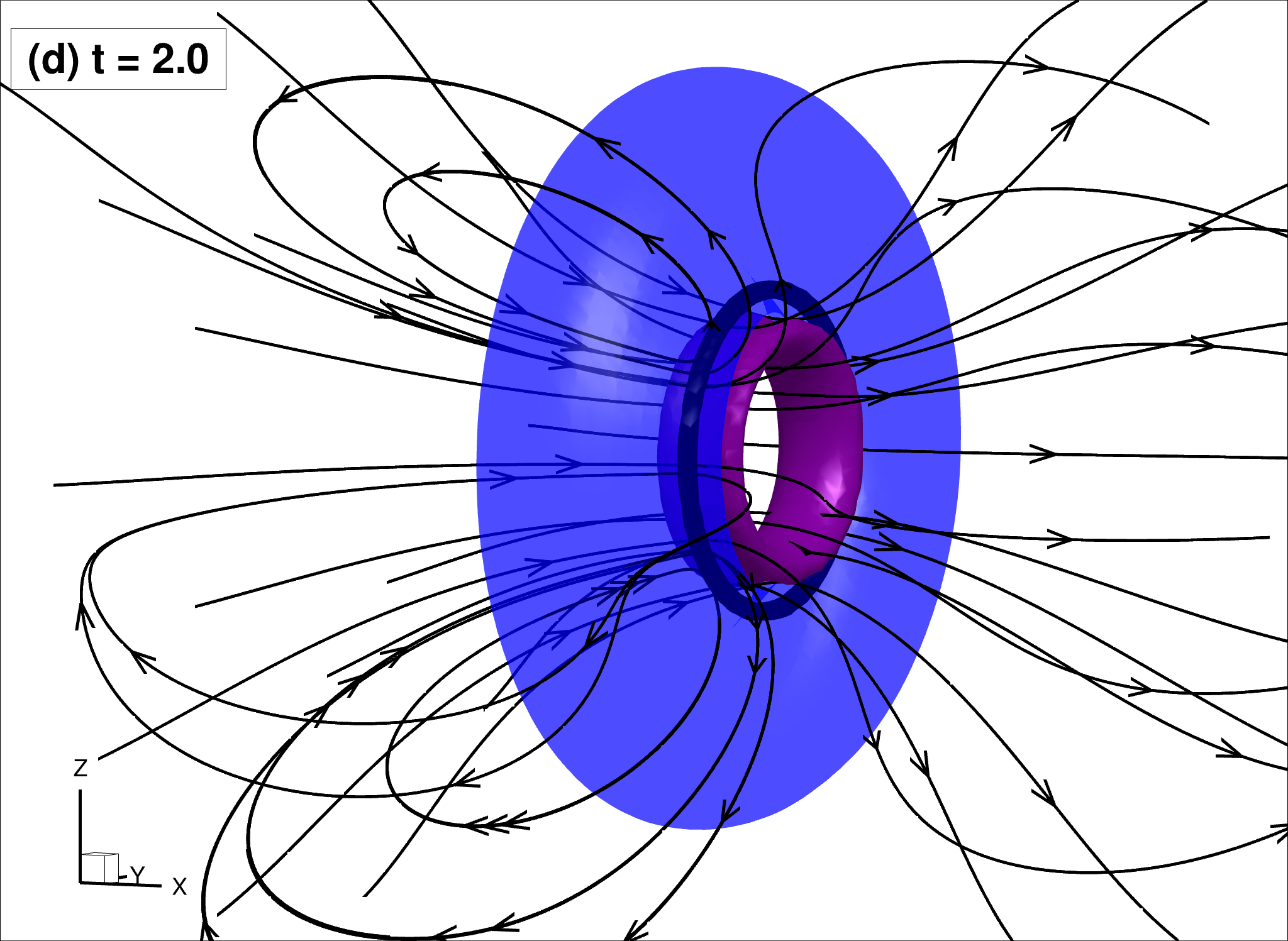
	$\rho_n/\rho_s = 1$ $B_{tab}=0.4 > B’_{tab} = 0.1$ $\eta_D=0.05 B_{tab}$
Snapshots of the flow for $t=0.7$	Snapshots of the flow for $t=2$

Supplemental material: structure of vortex reconnection

Test Case
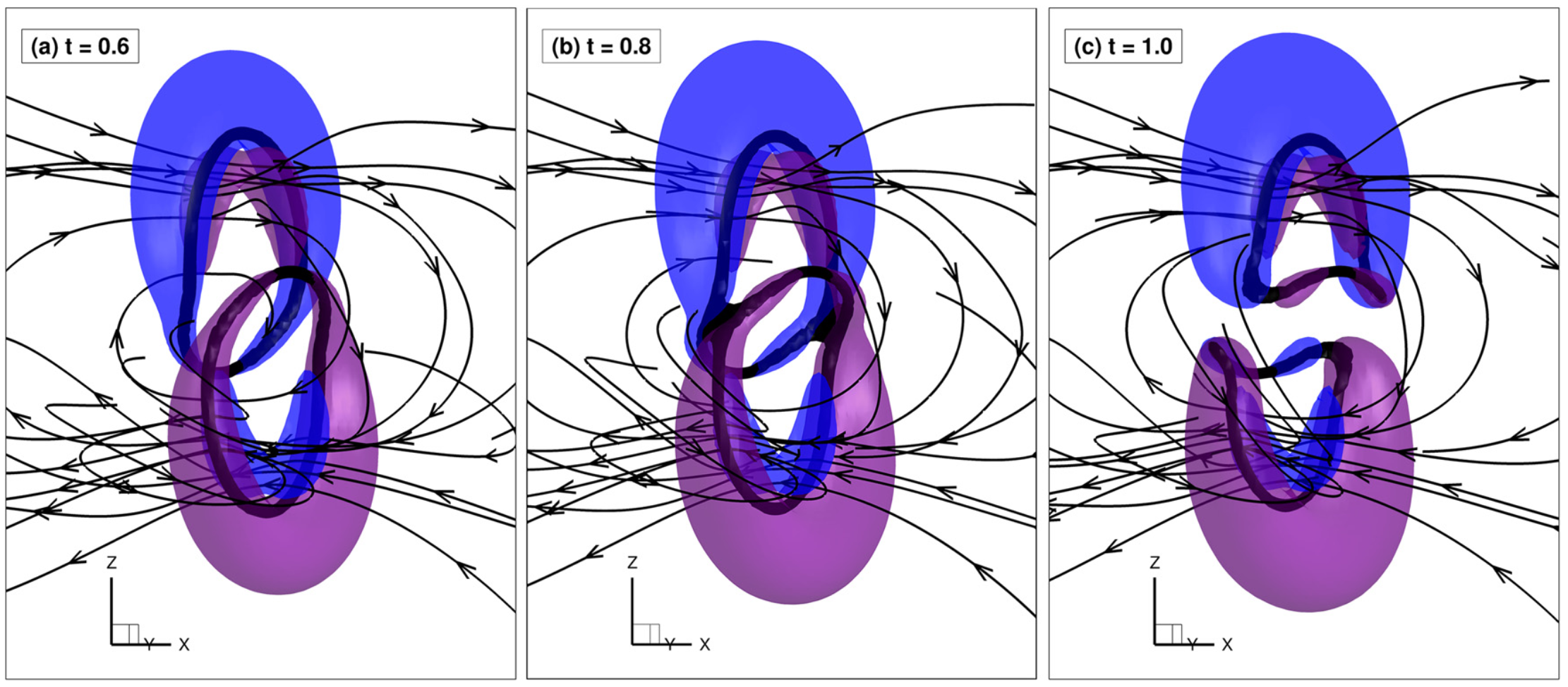
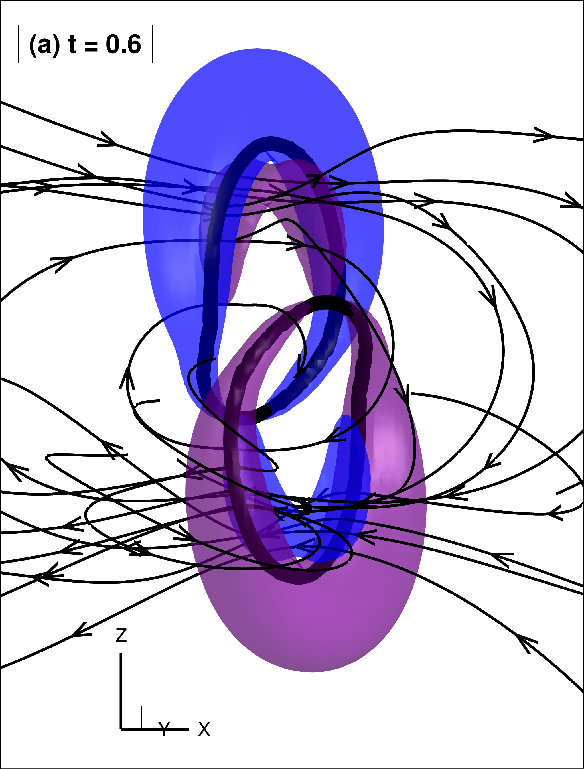
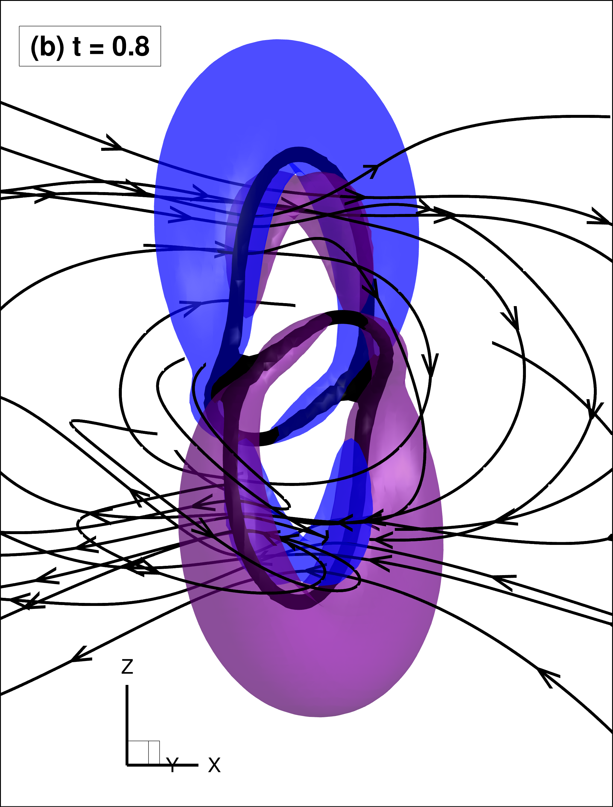
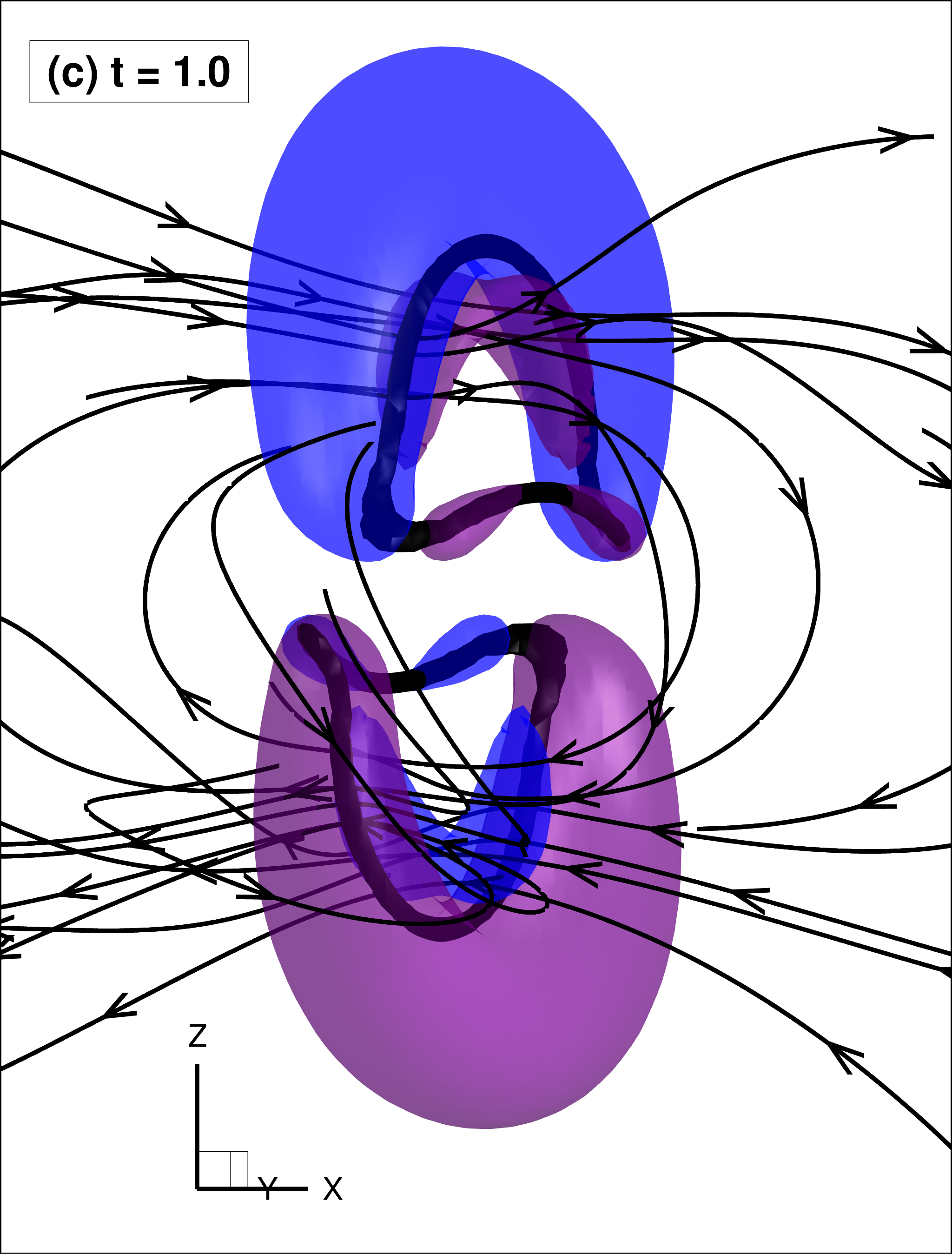
3D head-on collision of two superfluid vortex rings in a normal fluid initially at rest. Physical parameters $\rho_n/\rho_s = 1$, $B_{tab}=0.4$, $B’_{tab} = 0.1$, $\eta_D=0.05 B_{tab}$. The superfluid vortex ring (in black) is identified by an iso-surface of low atomic density (0.2 $\|\psi\|^2_{max}$). The two counter-rotating normal vortex rings are identified by iso-surfaces of normal fluid azimuthal vorticity: $0.05$ for the blue outer ring and ($-0.05$) for the red inner ring. The streamlines in the normal fluid are also drawn. Mesh resolution $128^3$.

3D head-on collision of two superfluid vortex rings in a normal fluid initially at rest. Physical parameters $\rho_n/\rho_s = 1$, $B_{tab}=0.4$, $B’_{tab} = 0.1$, $\eta_D=0.05 B_{tab}$. The superfluid vortex ring (in black) is identified by an iso-surface of low atomic density (0.2 $|\psi|^2_{max}$). The two counter-rotating normal vortex rings are identified by iso-surfaces of normal fluid azimuthal vorticity: $0.05$ for the blue outer ring and ($-0.05$) for the red inner ring. The streamlines in the normal fluid are also drawn. Mesh resolution $128^3$.


Snapshots of the flow for $t=0.6$	Snapshots of the flow for $t=.8$	Snapshots of the flow for $t=1$