Download preprint-pdf
Authors
G. Sadaka, A. Rakotondrandisa, P-H. Tournier, F. Luddens, C. Lothodé, I. Danaila
Abstract
We present and distribute a FreeFem++ Toolbox for the parallel computing of two- or three-dimensional liquid-solid phase-change systems involving natural convection. FreeFem++ (www.freefem.org) is a free finite-element software available for all existing operating systems. We use the recent library ffddm that makes available in FreeFem++ state-of-the-art scalable Schwarz domain decomposition methods (DDM). The single domain approach used in our previous contribution (A. Rakotondrandisa, G. Sadaka, I. Danaila, A finite-element Toolbox for the simulation of solid-liquid phase-change systems with natural convection, Computer Physics Communications, DOI 10.1016/j.cpc.2020.107188, 2020) is adapted for the use of the DDM method. As a result, the computational time is considerably reduced for 2D configurations and furthermore 3D problems become affordable. The numerical method is based on an enthalpy-porosity model. The same set of equations is solved in both liquid and solid phases: the incompressible Navier-Stokes equations with Boussinesq approximation for thermal effects. A Carman-Kozeny-type penalty term is added to the momentum equations to bring progressively the velocity to zero into the solid. Model equations are discretized using Galerkin triangular or tetrahedral finite elements. The coupled system of equations is integrated in time using a second-order Gear implicit scheme. The resulting discrete equations are solved using a Newton algorithm. The DDM approach is based on an overlapping Schwarz method. The mesh is first split in subdomains using Scotch or Metis libraries. The final linear system is then solved in parallel using a GMRES Krylov method, with a Restricted Additive Schwarz (RAS) preconditioner. The mesh is adapted during the computation using metrics control. The 3D-mesh adaptivity uses the mmg (www.mmgtools.org) open source library. Parallel 2D and 3D computations of benchmark cases of increasing difficulty are presented: natural convection of air, natural convection of water, melting or solidification of a phase-change material, and, finally, a water freezing case. For each case, careful validations are provided and the performance of the code is assessed. The robustness of the Toolbox in 3D is also demonstrated by adapting the number of processors to the number of tetrahedra, which can considerably vary after the mesh adaptation.
FreeFem++ Toolbox
Nature of problem: The software is scoped to parallel computations of 2D or 3D configurations of liquid-solid phase-change problems with convection in the liquid phase. Natural convection, melting and solidification processes are illustrated in the paper. The software can be easily modified to take into account different related physical models.
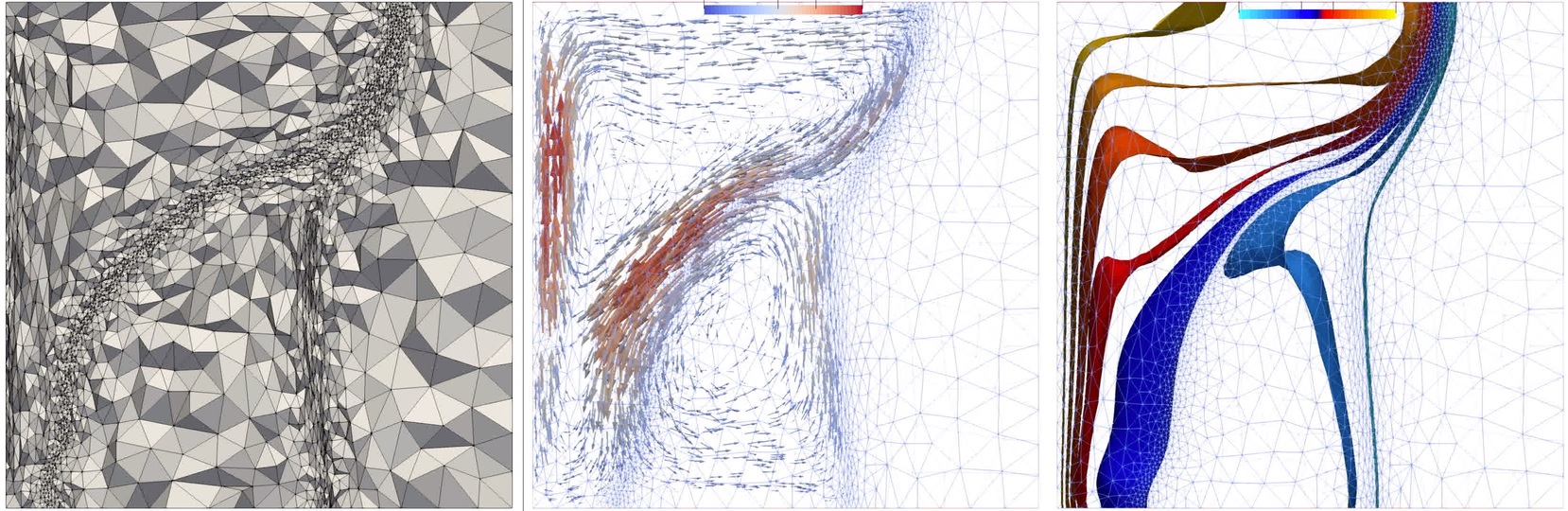
Solution method: We use a single domain approach, solving the incompressible Navier-Stokes equations with Boussinesq approximation in both liquid and solid phases. A Carman-Kozeny-type penalty term is added to the momentum equations to bring the velocity to zero into the solid phase. An enthalpy model is used in the energy equation to take into account the phase change. Discontinuous variables (latent heat, material properties) are regularized through an intermediate (mushy) region. Space discretization is based on Galerkin triangular/tetrahedral finite elements. A second order Gear implicit scheme is used for the time integration of the coupled system of equations. The resulting discrete equations are solved using a Newton algorithm. Piecewise quadratic (P2) finite-elements are used for the velocity and piecewise linear (P1) for the pressure. For the temperature both P2 or P1 discretization are possible. The mesh is first split in subdomains using Scotch or Metis libraries, which are interfaced with FreeFem++. Then, a Schwarz domain decomposition method is used through the FreeFem++ library ffddm. The final linear system is solved in parallel using a GMRES Krylov method, with a Restricted Additive Schwarz (RAS) preconditioner. Mesh adaptivity using metrics control makes possible the optimization of the distribution of mesh elements. For 3D case, the mmg open source library is used to adapt the mesh.
Running time: For 2D cases: from seconds for the natural convection case to minutes or hours for PCM melting or solidification. Using only 6 MPI processes (cores or threads) on a personal computer, the parallel computation can bring a speed-up of 1.3 to 3.97, depending on the difficulty of the problem.
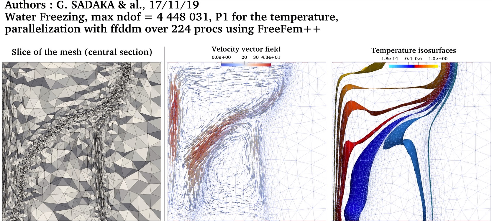
For 3D cases, the running time depends on the size of the problem and the number of processes: from 55 minutes for the unsteady natural convection of air with Ra=1e4 using 6 MPI processes to 1 day and 16h for the water freezing case using 224 MPI processes.
Supplemental material: parallel 2D simulations with DDM
| Test Case | Parameters |
|---|---|
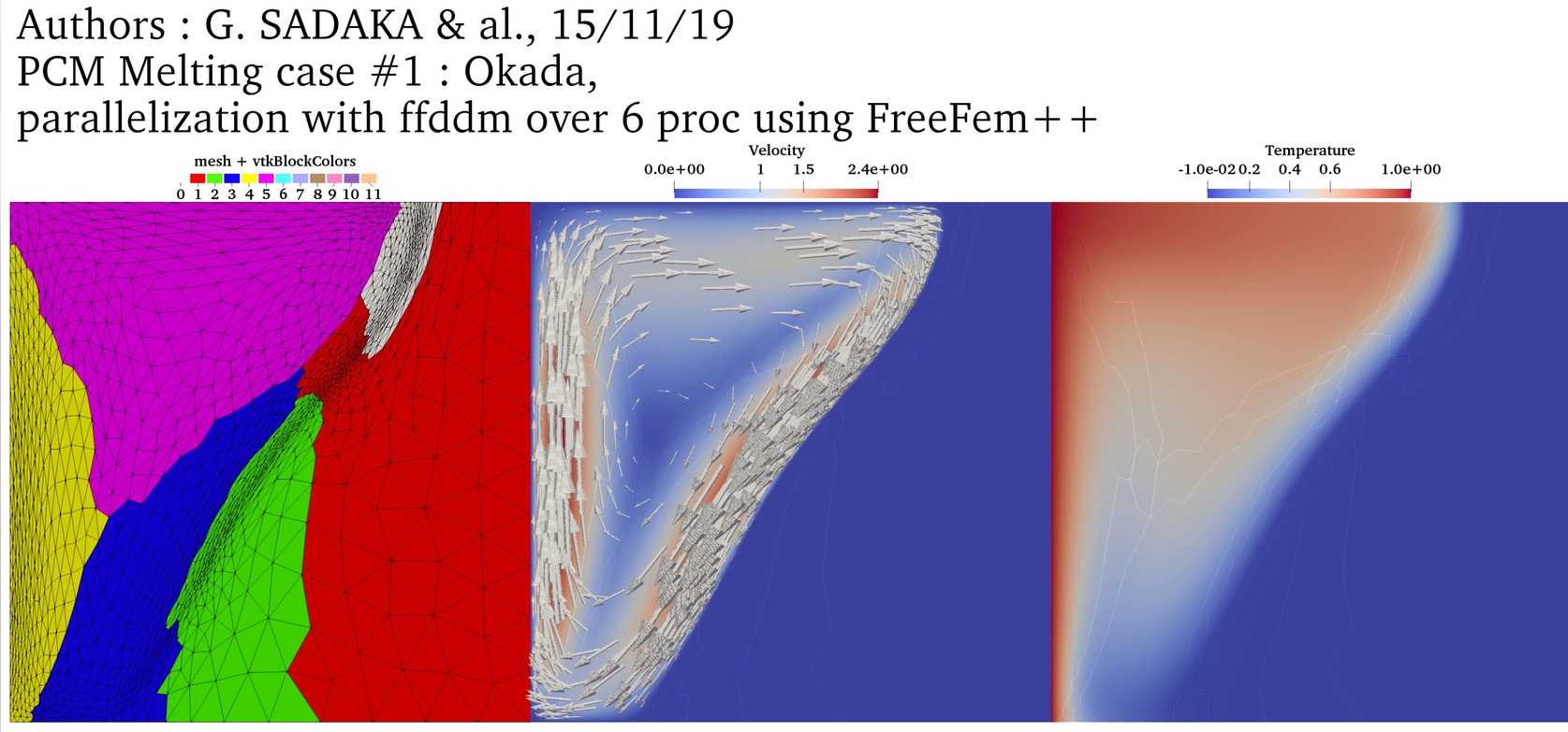
| 2D PCM Melting Case-1: Melting of a square PCM (Okada, 1984) |
$Ra = 3.27 \cdot 10^5$ $Pr = 56.2$ $Ste = 0.045$ $V_{ref} = \frac{\nu_l}{H}$ |
Temperature with P2 FE
➟ Download/Watch movie |
|
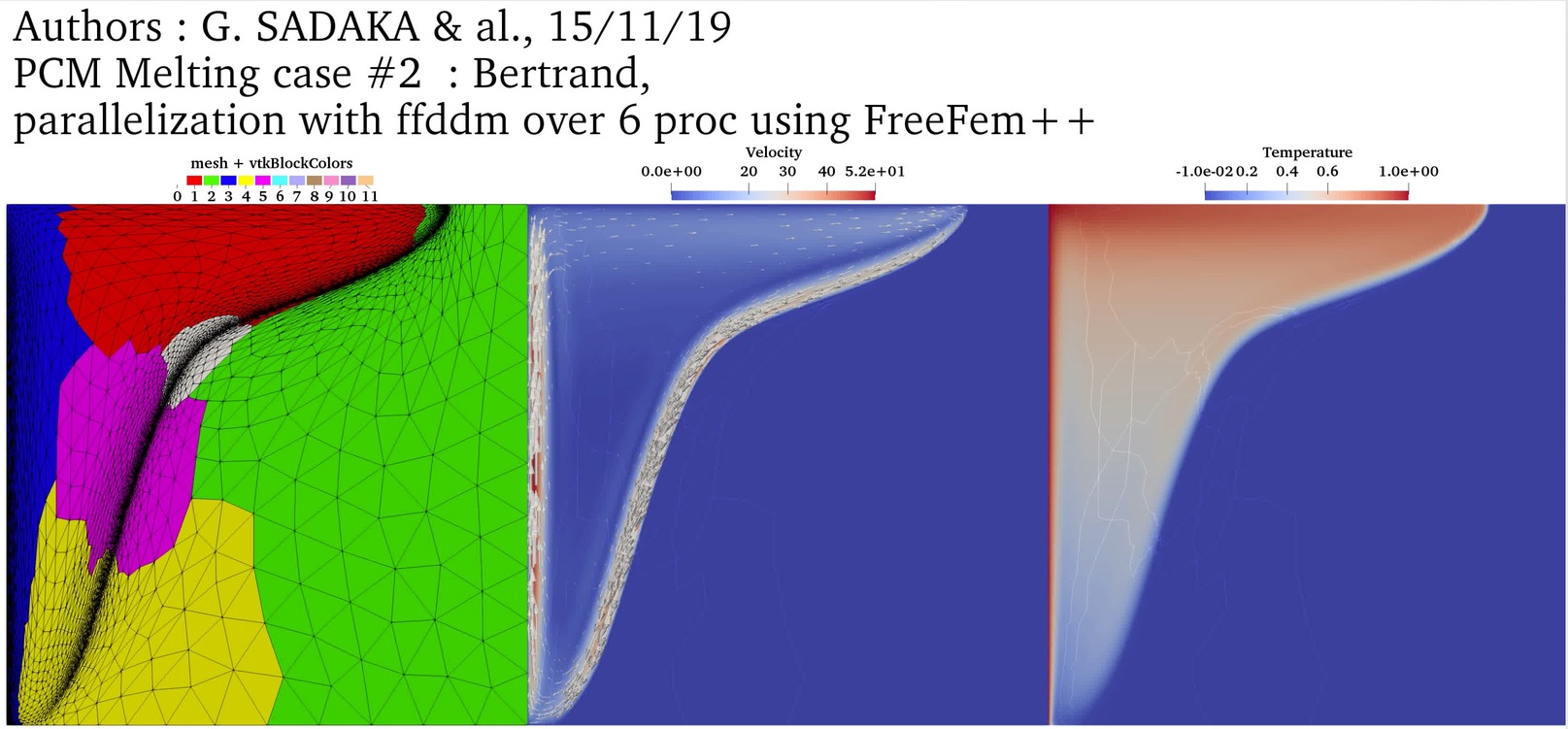
| 2D PCM Melting Case-2: Melting of a square PCM at high Rayleigh number (Bertrand et al., 1999) |
$Ra = 10^8$ $Pr = 50$ $Ste = 0.1$ $V_{ref} = \frac{\nu_l}{H}$ |
Temperature with P2 FE
➟ Download/Watch movie |
|
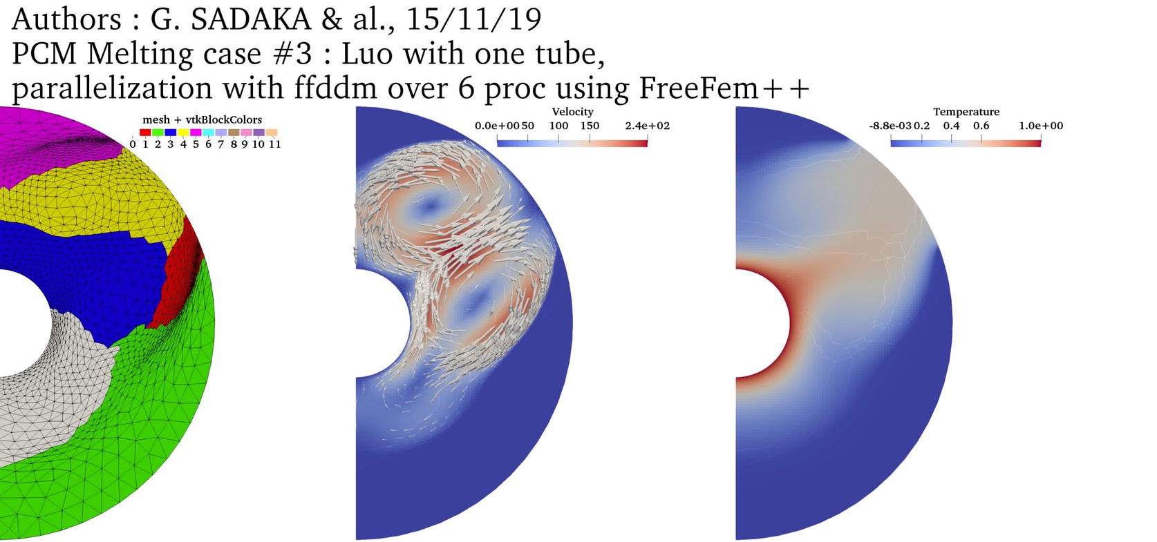
| 2D PCM Melting Case-3a: Melting of a circular PCM with one inner heated tube (Luo et al., 2015) |
$Ra = 5 \cdot 10^4$ $Pr = 0.2$ $Ste = 0.02$ $V_{ref} = \frac{\nu_l}{H}$ |
Temperature with P2 FE
➟ Download/Watch movie |
|
| 2D PCM Melting Case-3b: Melting of a circular PCM with four inner heated tube (Luo et al., 2015) |
$Ra = 5 \cdot 10^4$ $Pr = 0.2$ $Ste = 0.02$ $V_{ref} = \frac{\nu_l}{H}$ |
Temperature with P2 FE
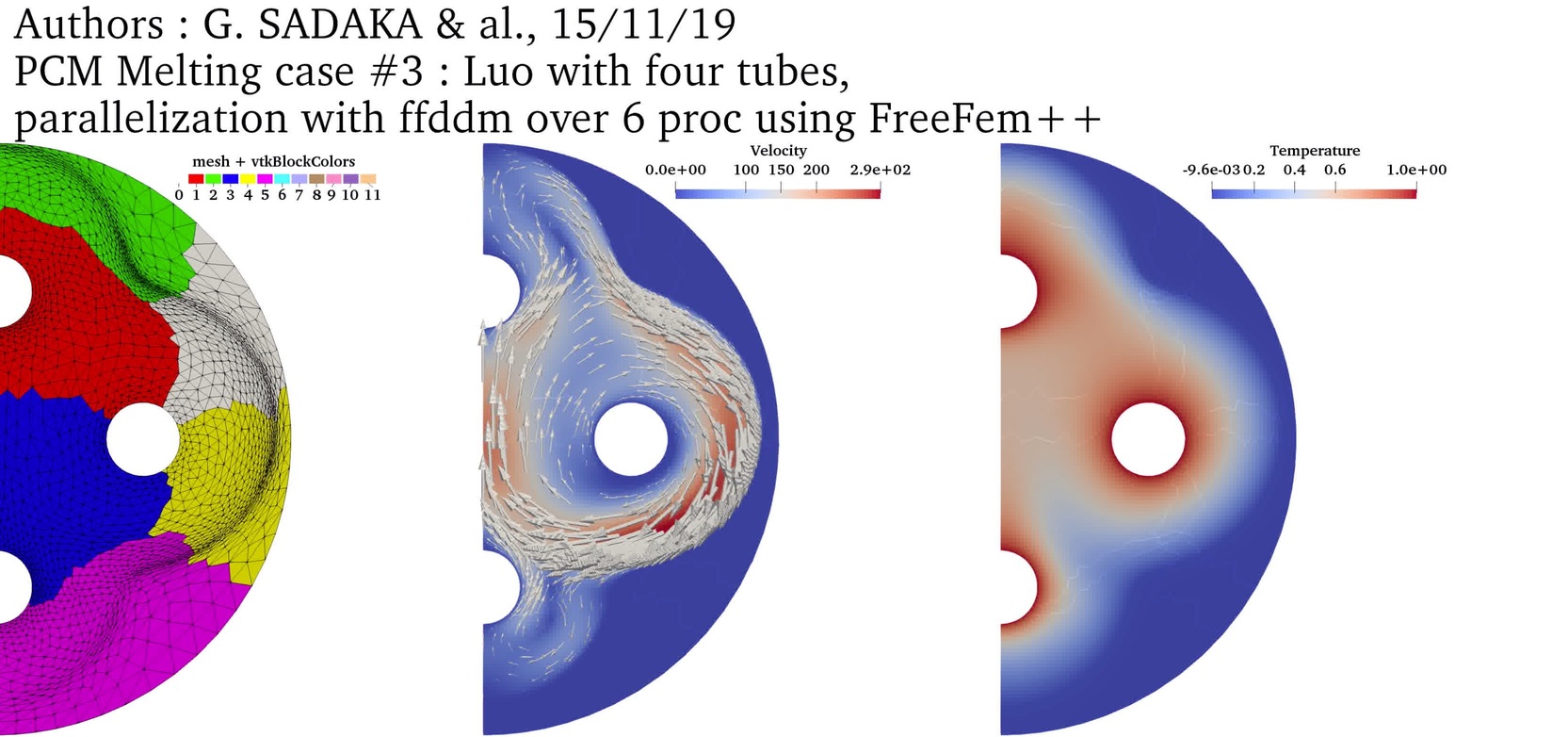
➟ Download/Watch movie |
|
| 2D PCM Melting Case-3c: Melting of a circular PCM with nine inner heated tube (Luo et al., 2015) |
$Ra = 5 \cdot 10^4$ $Pr = 0.2$ $Ste = 0.02$ $V_{ref} = \frac{\nu_l}{H}$ |
Temperature with P2 FE
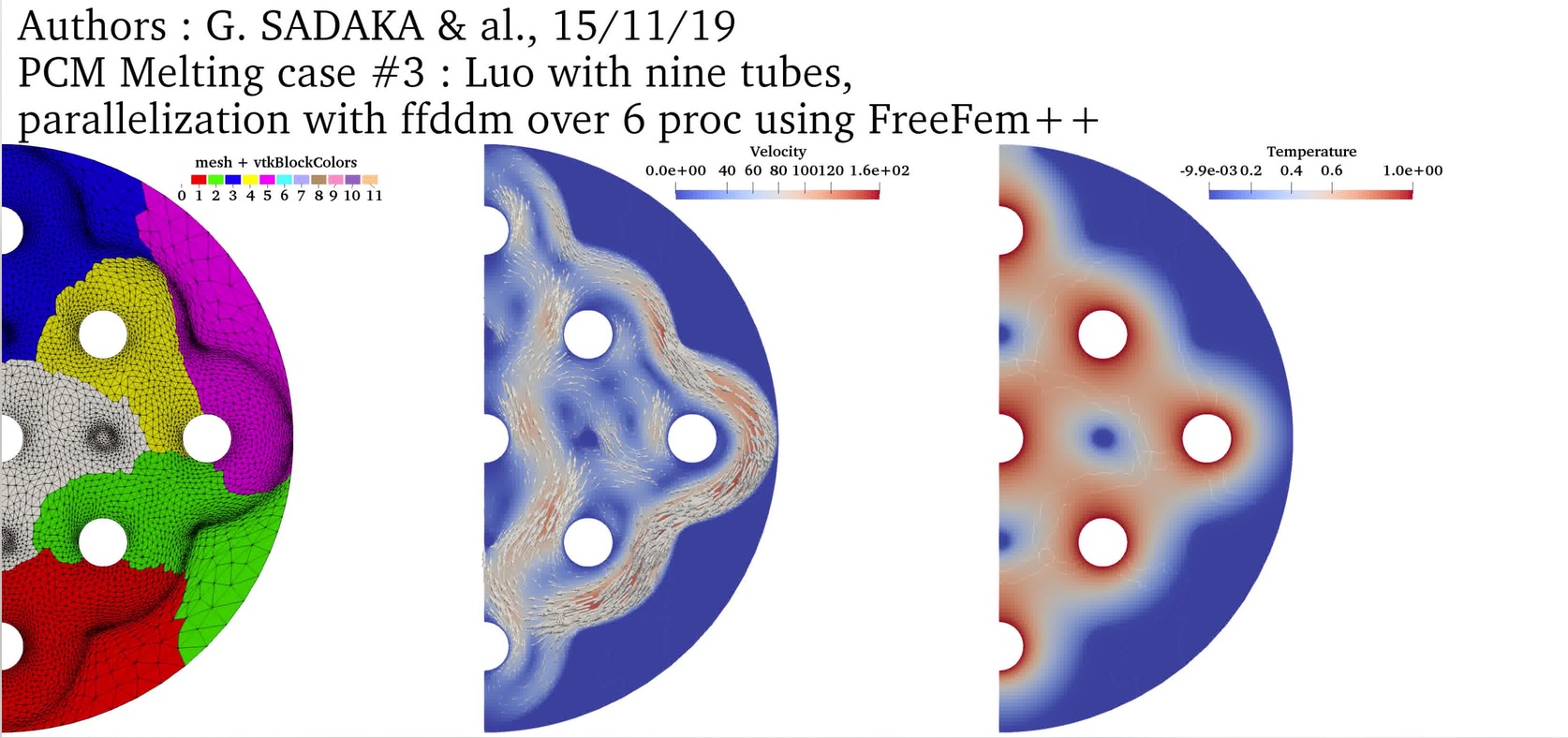
➟ Download/Watch movie |
|
| 2D PCM Melting Case-4: Melting of Gallium in a rectangular cavity (Hannoun et al., 2003) |
$Ra = 7 \cdot 10^5$ $Pr = 0.0216$ $Ste = 0.046$ $V_{ref} = \frac{\nu_l}{H}$ |
Temperature with P2 FE
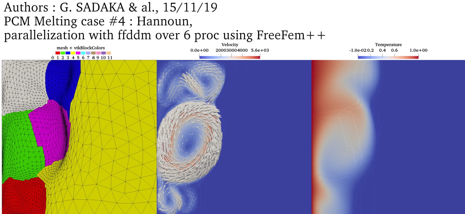
➟ Download/Watch movie |
|
| 2D PCM Melting Case-5: Solid crust formation in a highly distorted PCM (Nourgaliev et al., 2015) |
$Ra = 10^6$ $Pr = 0.1$ $Ste = 4.854$ $V_{ref} = \frac{\nu_l}{H} \sqrt{\frac{Ra}{Pr}}$ |
Temperature with P2 FE
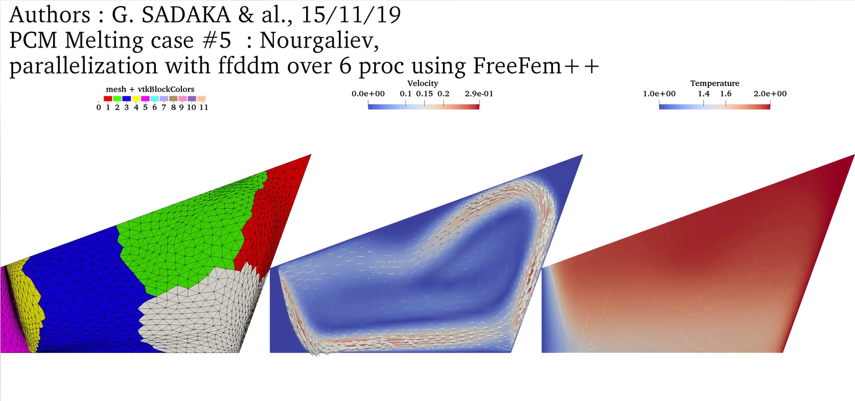
➟ Download/Watch movie |
|
| 2D Melting-solidification cycle: PCM Melting-1 (Okada, 1994) followed by the solidification from the left boundary |
$Ra = 3.27 \cdot 10^5$ $Pr = 56.2$ $Ste = 0.045$ $V_{ref} = \frac{\nu_l}{H}$ |
Temperature with P2 FE
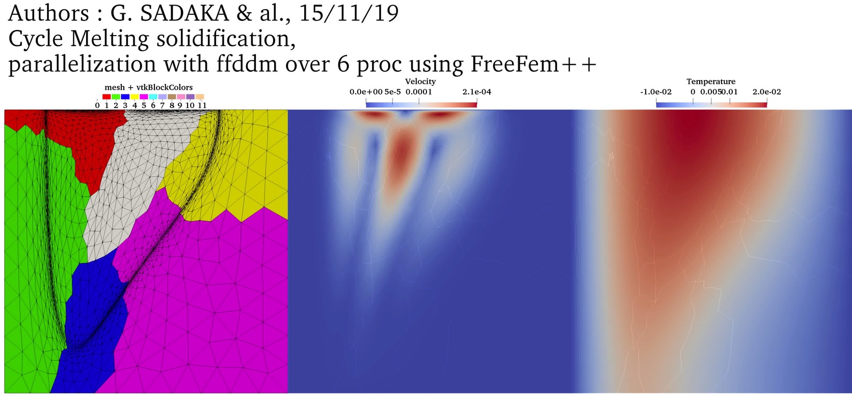
➟ Download/Watch movie |
|
| 2D Water freezing: the natural concetion state is first computed and then used as initial condition for simulating the freezing process |
$T_{left} = 10 ^oC$ (natural convection) $T_{right}= 0 ^oC$ (natural convection) $T_{left} = 10 ^oC$ (freezing) $T_{right}=-10 ^oC$ (freezing) |
Temperature with P2 FE
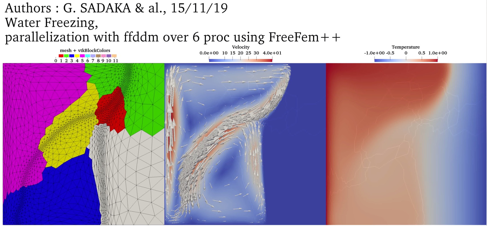
➟ Download/Watch movie |
Supplemental material: parallel 3D simulations with DDM
| Test Case | Parameters |
|---|---|
| 3D PCM Melting Case-1: Melting of a square PCM (Okada, 1984) |
$Ra = 3.27 \cdot 10^5$ $Pr = 56.2$ $Ste = 0.045$ $V_{ref} = \frac{\nu_l}{H}$ |
Temperature with P2 FE
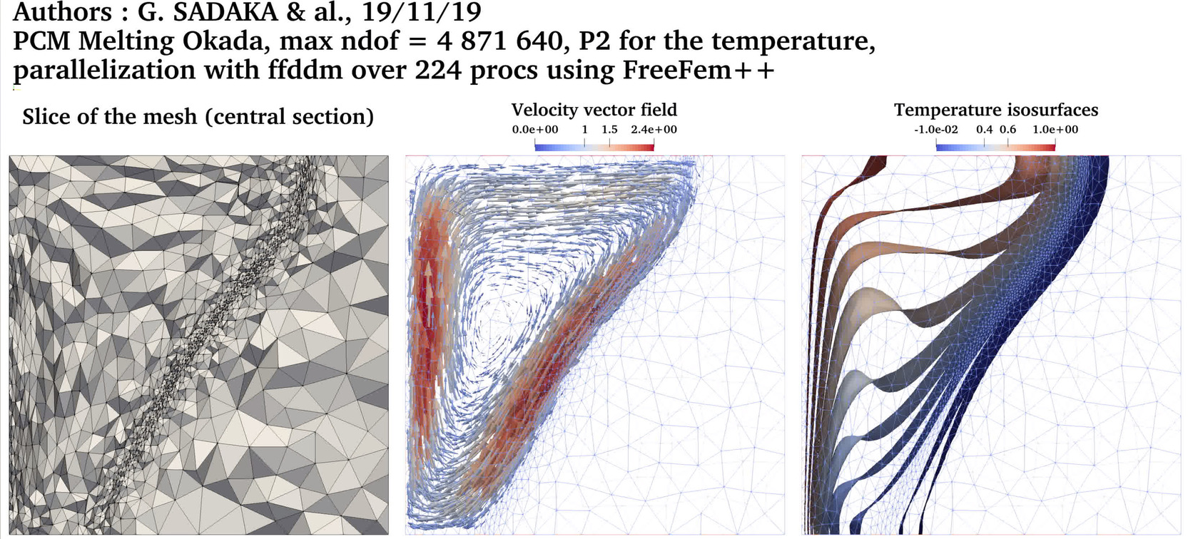
➟ Download/Watch movie |
Temperature with P1 FE
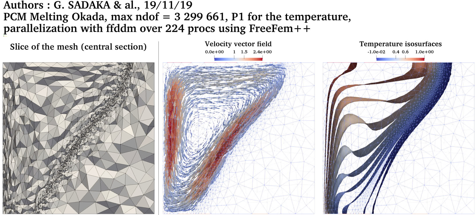
➟ Download/Watch movie |
| 3D PCM Melting Case-3a: Melting of a circular PCM with one inner heated tube (Luo et al., 2015) |
$Ra = 5 \cdot 10^4$ $Pr = 0.2$ $Ste = 0.02$ $V_{ref} = \frac{\nu_l}{H}$ |
Temperature with P2 FE
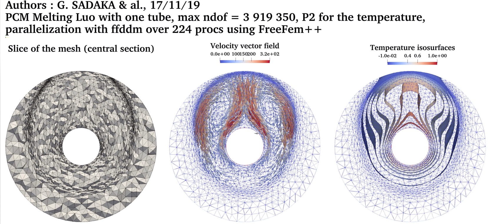
➟ Download/Watch movie |
Temperature with P1 FE
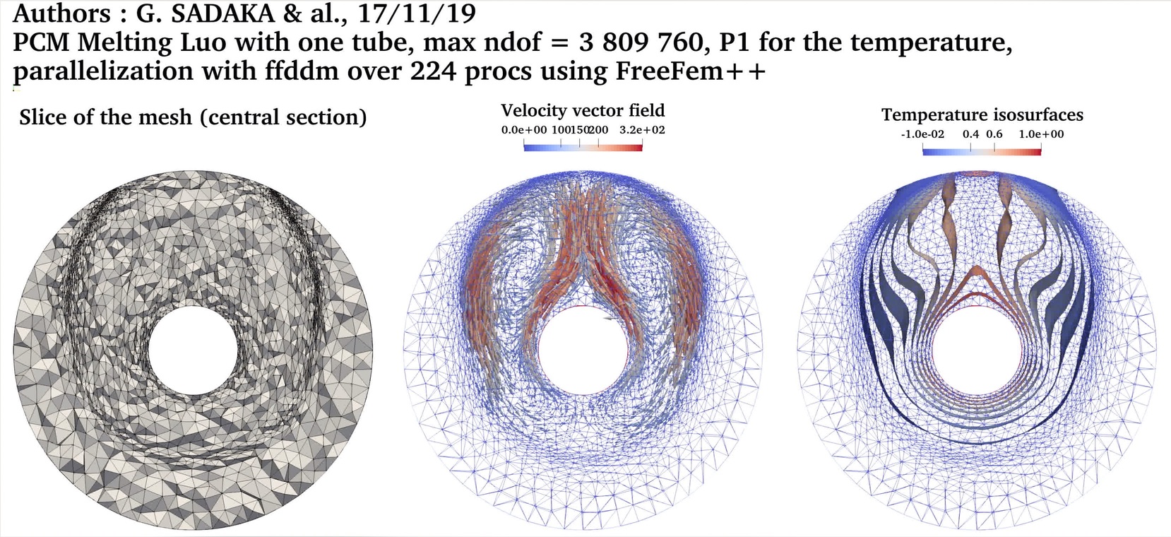
➟ Download/Watch movie |
| 3D PCM Melting Case-3b: Melting of a circular PCM with four inner heated tube (Luo et al., 2015) |
$Ra = 5 \cdot 10^4$ $Pr = 0.2$ $Ste = 0.02$ $V_{ref} = \frac{\nu_l}{H}$ |
Temperature with P2 FE
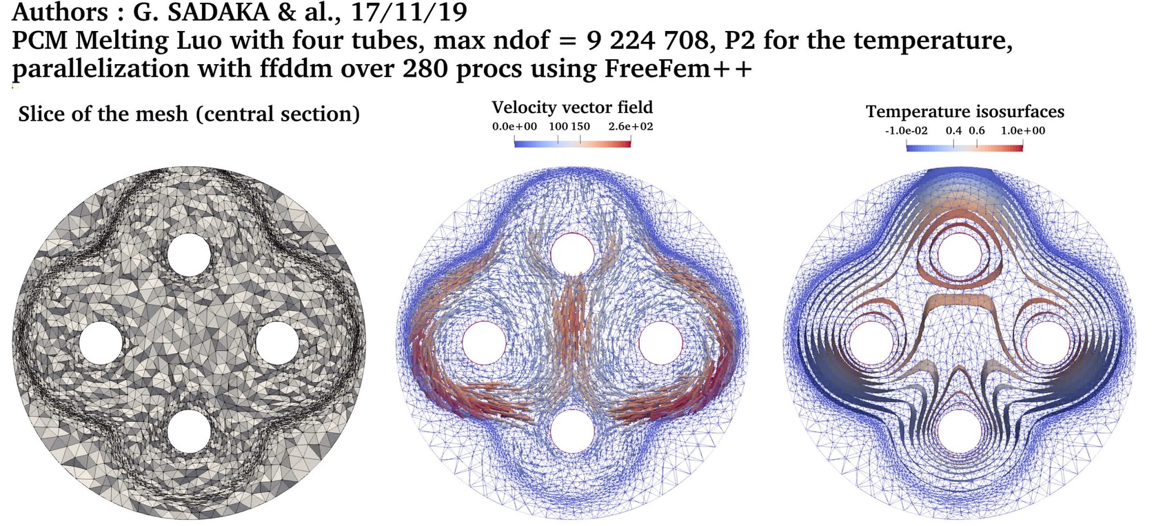
➟ Download/Watch movie |
Temperature with P1 FE
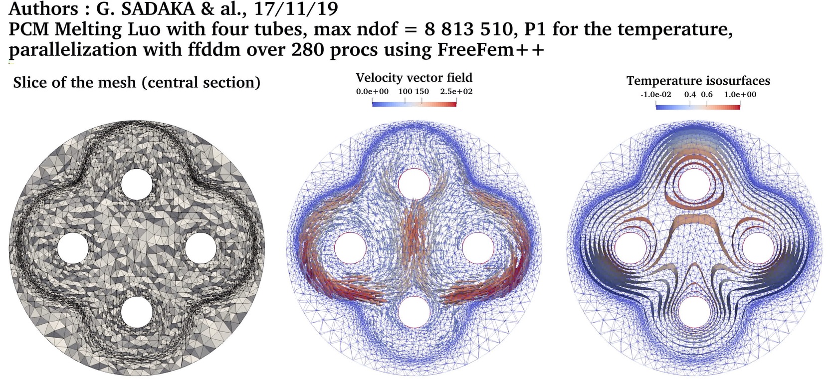
➟ Download/Watch movie |
| 3D PCM Melting Case-3c: Melting of a circular PCM with nine inner heated tube (Luo et al., 2015) |
$Ra = 5 \cdot 10^4$ $Pr = 0.2$ $Ste = 0.02$ $V_{ref} = \frac{\nu_l}{H}$ |
Temperature with P2 FE
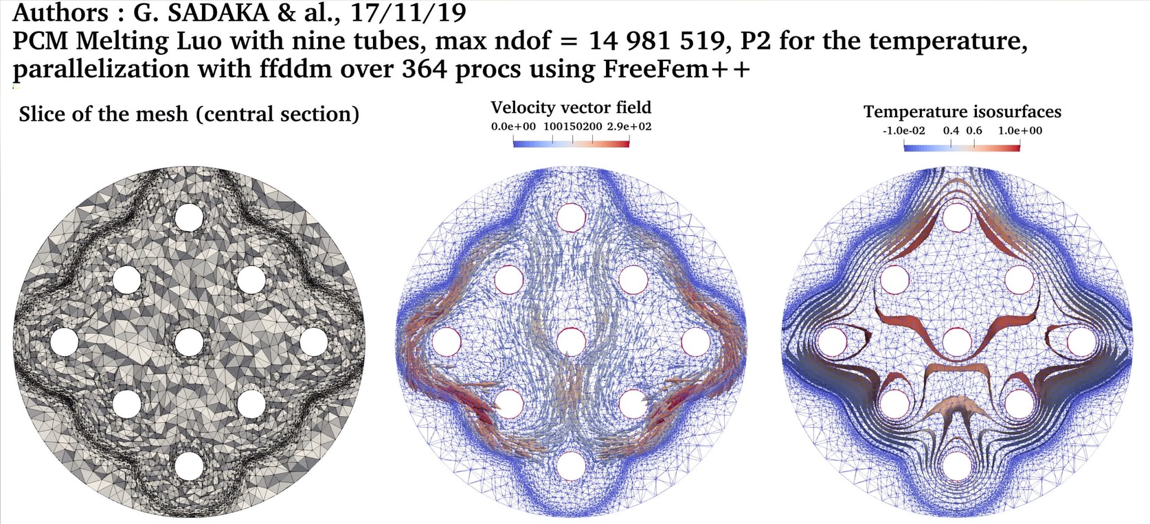
➟ Download/Watch movie |
Temperature with P1 FE
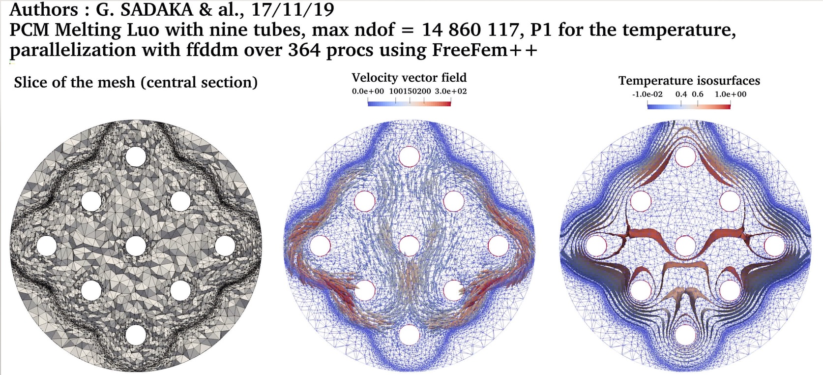
➟ Download/Watch movie |
| 3D Melting-solidification cycle: PCM Melting-1 (Okada, 1994) followed by the solidification from the left boundary |
$Ra = 3.27 \cdot 10^5$ $Pr = 56.2$ $Ste = 0.045$ $V_{ref} = \frac{\nu_l}{H}$ |
Temperature with P2 FE
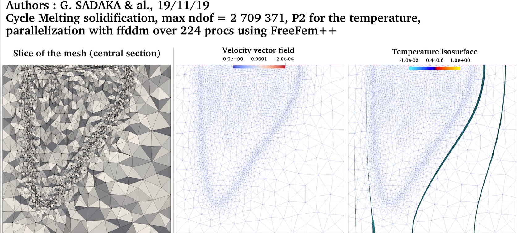
➟ Download/Watch movie |
Temperature with P1 FE

➟ Download/Watch movie |
| 3D Water freezing: the natural concetion state is first computed and then used as initial condition for simulating the freezing process |
$T_{left} = 10 ^oC$ (natural convection) $T_{right}= 0 ^oC$ (natural convection) $T_{left} = 10 ^oC$ (freezing) $T_{right}=-10 ^oC$ (freezing) |
Temperature with P2 FE
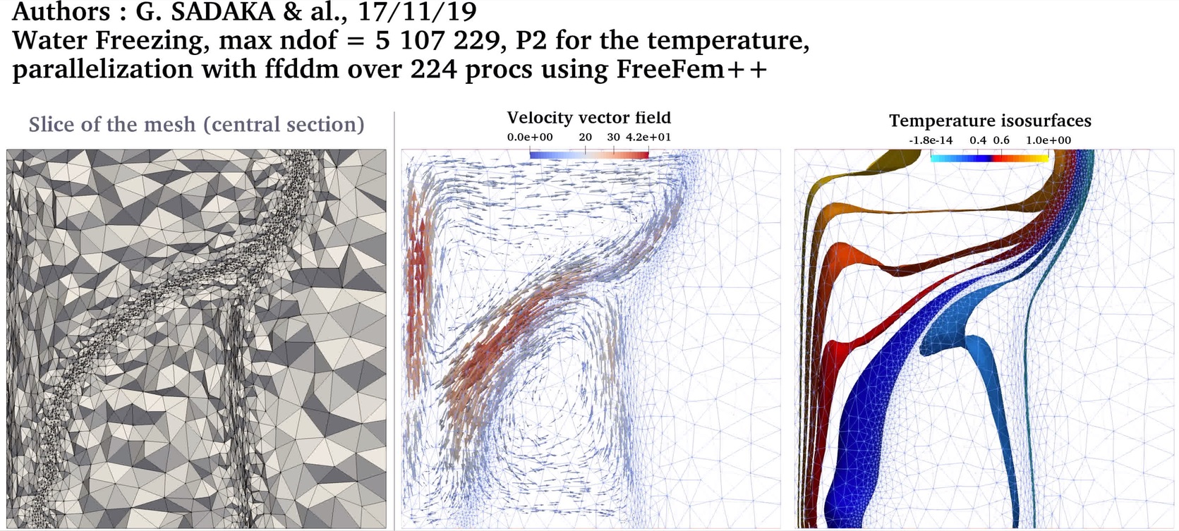
➟ Download/Watch movie |
Temperature with P1 FE
➟ Download/Watch movie |