Context
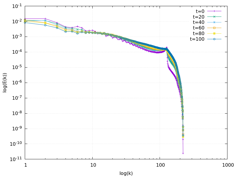
This topic is part of the new ANR project QUTE-HPC. Using the home made software GPS (Gross Pitaevskii Simulator), we start simulating simple configurations for QT. This requires the implementation of suitable boundary conditions and diagnostics to study energy spectra.
QT is modeled using the time-dependent Gross-Pitaevskii equation (in dimension less form): $$\begin{array}{rcl} -i\partial_t \psi &=& \frac12\Delta\psi - V(x)\psi - \beta |\psi|^2\psi \\ \psi_{|t=0} &=& \psi_0. \end{array}$$
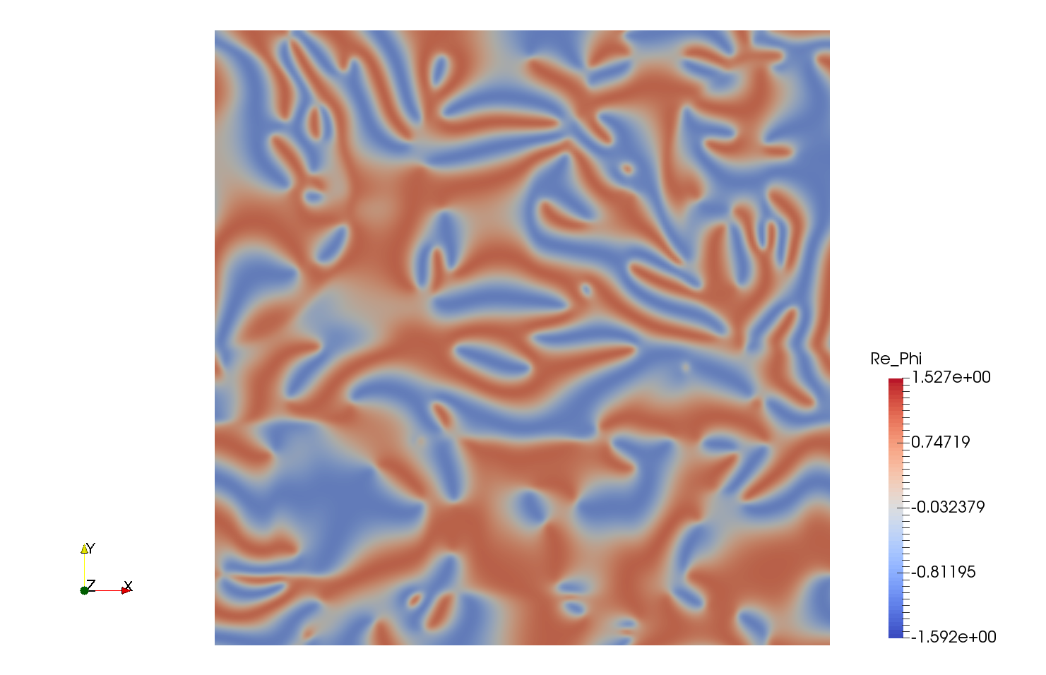
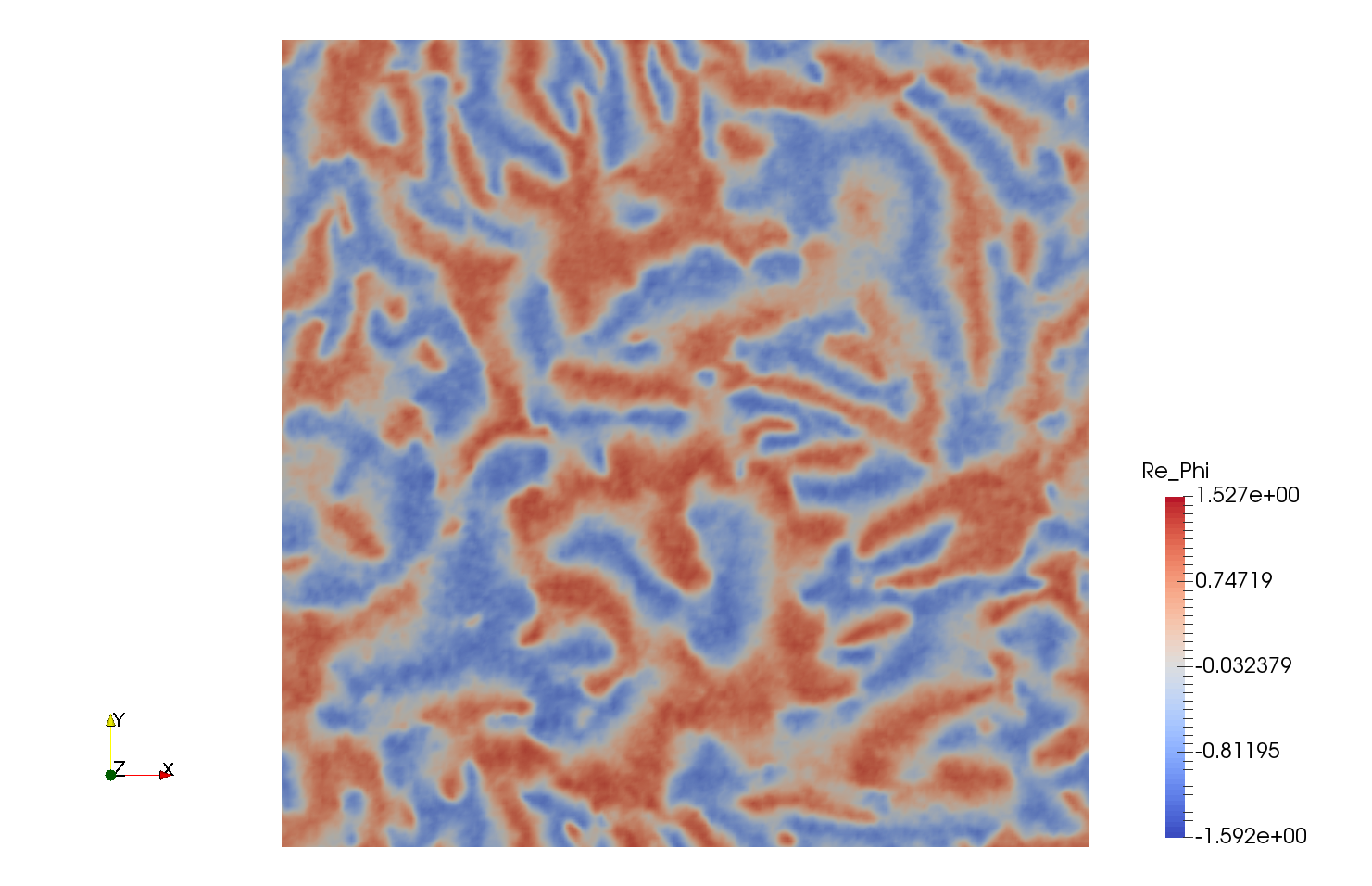
Different choices for $\psi_0$ are investigated to study the mechanisms of QT. A first choice is $\psi_0=e^{i\theta}$ where $\theta$ is a (smoothed) random phase field. A second choice is to introduce vortex rings pairs in a constant initial state. The last one is adapted from $cite?$
Tools
We use our home made software GPS:
- written in Fortran,
- hybrid MPI/OpenMP code,
- spatial discretization: spectral or high order compact finite differences scheme,
- 2nd order time-splitting scheme.
Results
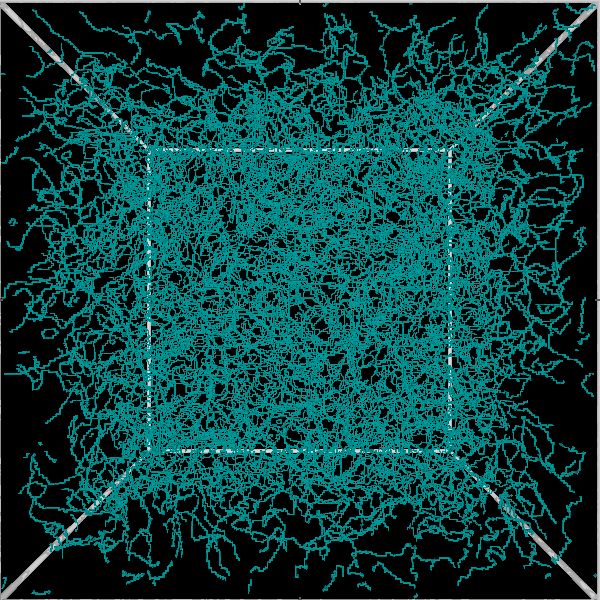 Final state for quantum turbulence: initial state contains 100 pairs of vortex rings. Click here to see the time evolution of the vortices.